First let us understand the difference between OCV and PVT.

OCV - on chip variations PVT - Process, Voltage, Temparature variations.

PVT are inter-chip variations, which largely depend on external factors like: temp, voltage, and process of that particular chip at the time of manufacturing. Like PVT, OCV’s are also variation in voltage, temp, process but OCVs are intra chip variations.

Now let us understand the difference between OCV and AOCV. The semiconductor device manufacturing process exhibits two kinds of variations.

1. Systemic variations:

• Systematic variations are deterministic in nature and these can be usually attributed to a particular manufacturing process parameter like manufacturing equipment used or even manufacturing technique used. Systematic variations could be experimentally calibrated and modelled. They also exhibit spacial correlation, which means if two transistors are close , they experience simialr variation.

2. Random variations: These are totally random therefore they are non deterministic in nature. Random variation does not show any spatial correlation so they are hard to gauge and predict.

OCV and AOCV are models which guide us on how the cell delay varied in light of systematic and random variations.

On-chip variations (OCV): Are simplistic variations and usally modelled as pessimistic. As long as the process guys can ensure that the variation is withing +x% and -x% , we applying +X and -X% pessimistic delays to cells will help model the variations.

Setup Ananlysis under OCV: Inorder make the setup analysis immnue to process variations , we need to model the OCV’s such that setup check becomes pessimistic. That would be the case if we increase the datapath delay by x% , increase the launch clock path delay by x% and reduce the capture clock path delay by x%

Hold Analysis under OCV: This is going to be exact opposite. i.e decrease the data path delay by x%, decrease the launch clock path delay by x% and increase the launch clock path delay by x%.

Advanced on0chip variations (AOCV)

• Cell Type Variations should take into account the cell type. The impact of variation shld be calculated for each individual cell.
• Distance As the distance in X-Y coordinates increase, the systematic variations increase and we might need to use higher derate value to mitigate the variation in silicon.
• Path Depth If within a given distance, if path depth is more, the impact of Systematic variations could be constant, but the random variations tend to cancel each other. Therefore as the path depth increase (within a unit distance) , the AOCV derates tend to decrease.

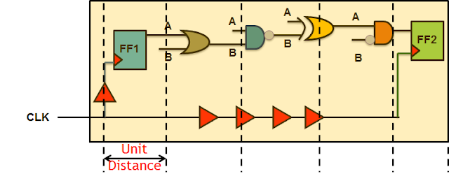
While performing reg2reg timing analysis, AOCV mehtodology finds the bounding box containing the sequentials, clock buffers between sequentials and all the data cells. Within a unit distance, if the path depth increases - AOCV derate decreases due to cancelling of random vvariation. but, if the distance increases, AOCV derate increases due to increase in systematic variations. Therefore, variations are modelled in LUT form:

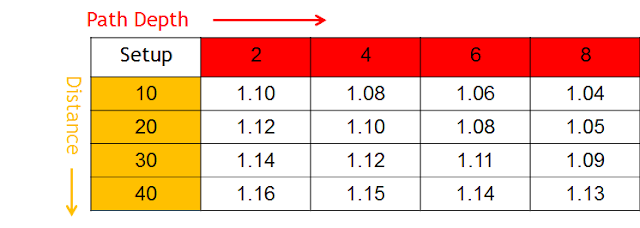
For small path depths, OCV seem to be optimistic. AOCV is more accurate. For higher path depths, OCV tends to be more pessimistic. AOCV is more accurate.

From another article

Advanced on-chip variation (AOCV) analysis reduces unnecessary pessimism by taking the design methodology and fabrication process variation into account. AOCV determines derating factors based on metrics of path logic depth and the physical distance traversed by a particular path. A longer path that has more gates tends to have less total variation because the random variations from gate to gate tend to cancel each other out. A path that spans a larger physical distance across the chip tends to have larger systematic variations. AOCV is less pessimistic than a traditional OCV analysis, which relies on constant derating factors that do not take path-specific metrics into account.

The AOCV analysis determines path-depth and location-based bounding box metrics to calculate a context-specific AOCV derating factor to apply to a path, replacing the use of a constant derating factor.

AOCV analysis works with all other PrimeTime features and affects all reporting commands. This solution works in both the Standard Delay Format (SDF)-based and the delay calculation based flows.

Compared to AOCV, POCV provides

•Reduced pessimism gap between graph-based analysis and path-based analysis

Parametric on-chip variation (POCV) analysis can be performed in graph-based analysis (GBA) or path-based analysis (PBA) mode, depending on the -pba_mode setting of the report_timing or get_timing_paths command.

What is the difference between GBA POCV and PBA POCV when the pba_derate_only_mode variable is set to true?

POCV uses a Gaussian distribution to model “random variation,” whereas it uses distance-based derating to model “systematic variation” (similar to AOCV). Two key parameters in POCV random variation modeling are the mean (average delay) and sensitivity (standard deviation or sigma). Sensitivity is derived from side file or Liberty Variation Format (LVF) data.

In the default PBA mode, PrimeTime performs two path-based recalculation processes: slew recalculation and derating recalculation. However, when the variable pba_derate_only_mode variable is set to true, only derating recalculation is performed.

In GBA POCV, each object (cell and net) is typically part of many different paths, and the tool computes distance metrics conservatively for each object to avoid optimism for any single path. With derate-only mode enabled, PBA POCV only removes the only pessimism resulting from “systematic variation” (distance-based derating); the “random variation” pessimism of GBA POCV is the same as for PBA POCV.